> ##### [R Distributions] #####
> ##### 1. Binomial Distributions : 이항분포 #####
>
> # 1) pmf을 이용한 확률 계산
> p <- 1/3; n <- 3; x <- 1 # 확률 1/3, 시행횟수 3회일 때 1회 성공할 확률
> choose(n, x) * (p)^x * (1-p)^(n-x) # 이항분포 공식: nCx * p^x * (1-p)^(n-x)
[1] 0.4444444
>
> p <- 1/3; n <- 3; x <- 0:3 # 확률 1/3, 시행횟수 3회일 때 0~3회 성공할 확률분포
> choose(n, x) * (p)^x * (1-p)^(n-x)
[1] 0.29629630 0.44444444 0.22222222 0.03703704
>
> # 2) dbinom 함수를 이용한 확률 계산
> dbinom(1, size=n, prob=p) # dbinom = d(밀도함수) + binom(이항분포) = density + binomial
[1] 0.4444444
> (binom.pdf <- dbinom(0:n, size=n, prob=p)) # 전체 확률밀도 분포, 전체괄호 시 즉시 실행
[1] 0.29629630 0.44444444 0.22222222 0.03703704
>
> # 3) dbinom 함수와 cumsum 함수를 이용한 누적확률 계산
> cumsum(binom.pdf) # 전체 누적확률분포 계산 = cum(누적분포) + sum(합)
[1] 0.2962963 0.7407407 0.9629630 1.0000000
>
> # 4) pbinom 함수를 이용한 누적확률 계산
> (binom.cdf <- pbinom(0:n, size=n, prob=p)) # 전체 누적확률분포 (cdf; cumulative distribution function)
[1] 0.2962963 0.7407407 0.9629630 1.0000000
>
> # 5) 이항난수 발생
> set.seed(968) # 추출될 난수 고정
> n = 100; p = 0.3
> (binom.rnd <- rbinom(20, size=n, prob=p)) # 난수 추출
[1] 35 30 23 29 36 30 32 32 31 25 20 28 33 36 27 25 37 31 27 29
> table(binom.rnd) # 추출된 난수를 테이블로 생성
binom.rnd
20 23 25 27 28 29 30 31 32 33 35 36 37
1 1 2 2 1 2 2 2 2 1 1 2 1
>
> # 6) 기대치와 분산
> n * p # E(X) = np; 모평균 = 기댓값
[1] 30
> mean(binom.rnd) # 추출된 값의 평균; 이항난수 평균
[1] 29.8
> n * p * (1-p) # V(X) = np(1-p) = npq; 모분산
[1] 21
> var(binom.rnd) # 추출된 값의 분산; 이항난수 분산
[1] 20.37895
> cnt <- c(10, 30, 100, 1000, 10000, 50000) # 난수 추출 개수
> E <- sapply(cnt, FUN=function(cnt) # 추출 개수별 평균
+ mean(rbinom(n=cnt, size=n, prob=p)))
> V <- sapply(cnt, FUN=function(cnt) # 추출 개수별 분산
+ var(rbinom(n=cnt, size=n, prob=p)))
> data.frame(E, V)
E V
1 30.30000 27.73333
2 30.50000 18.60230
3 30.13000 21.49455
4 30.16000 21.55591
5 30.04060 20.96938
6 29.99634 21.14781
> opar <- par(mfrow = c(1,2))
> hist(E, main ="Histogram of Binomial: Mean", col='#FF0000')
> hist(V, main ="Histogram of Binomial: Var", col=rgb(0,0,1)) # 이항분포의 히스토그램
> par(opar)

> # 7) CDF: 누적분포함수
> n <- 15; p.1 <- 1/4; p.2 <- 2/4; p.3 <- 3/4
> n * p.1
[1] 3.75
> pbinom(5, n, p.2) # P(X<=5) = Sigma x=0~10, [(15Cx) * 0.5^x * (1-0.5)^x]
[1] 0.1508789
> pbinom(10, n, p.3)-pbinom(9, n, p.3) # P(X=10) = P(X<=10)-P(X<=9) = Sigma x=0~10, [(15Cx) * 0.75^x * (1-0.25)^x]
[1] 0.165146
> dbinom(10, n, p.3) # P(X=10) = Sigma x=0~10, [(15Cx) * 0.75^x * (1-0.25)^x]
[1] 0.165146
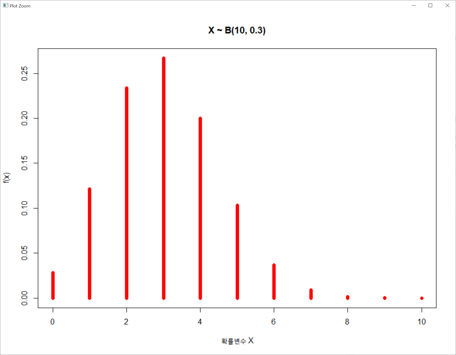
> ##### 실습1. 이항분포 밀도함수 #####
> # 성공확률 p인 베르누이 시행을 n회 했을 때
> y <- dbinom(0:10, size=10, prob=0.3) # dbinom = d(밀도함수) + binom(이항분포) = density + binomial
> plot(0:10, y, type='h', col='Red', ylab='f(x)', xlab='확률변수 X', lwd=7,
+ main = c("X ~ B(10, 0.3)"))
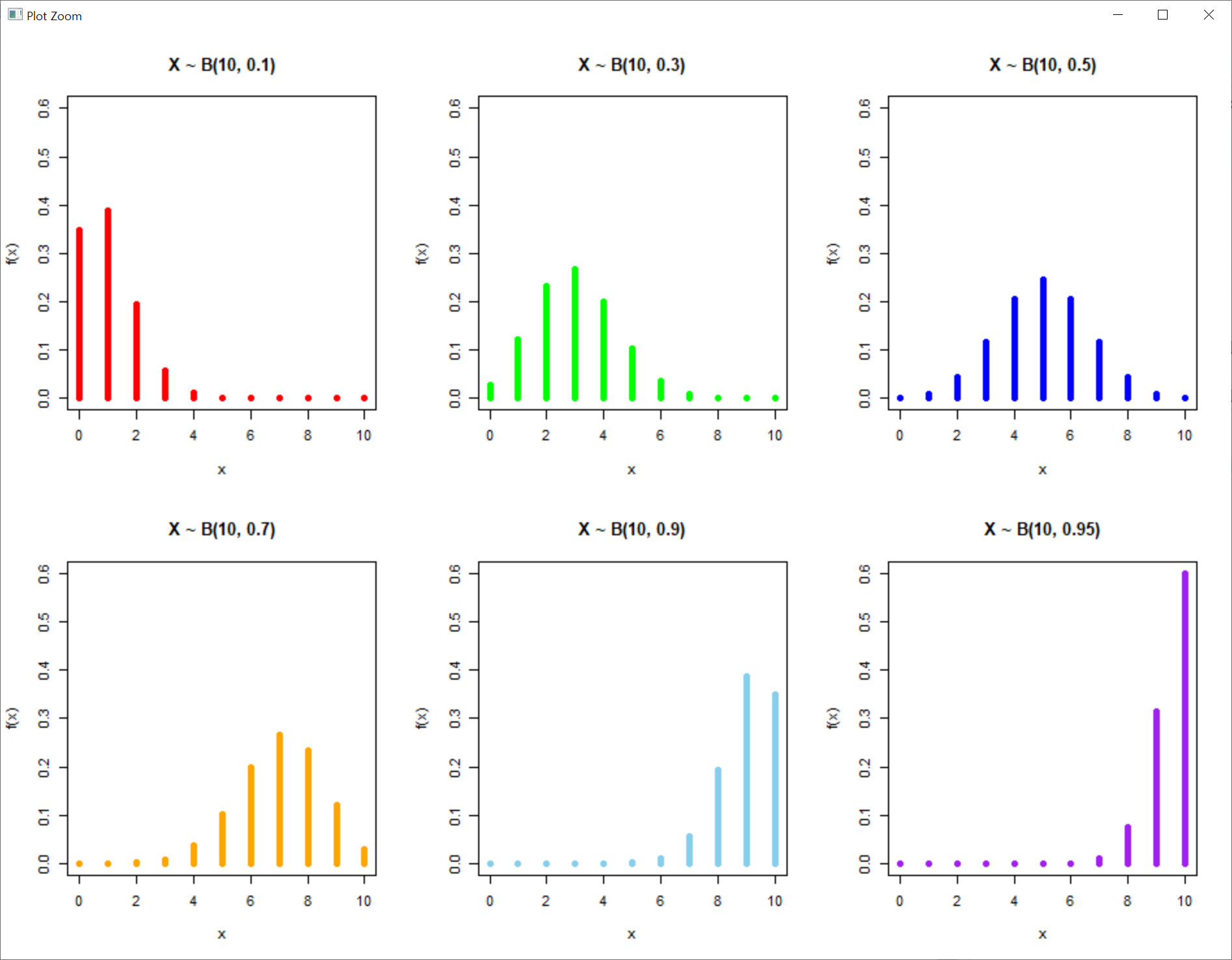
> # (1) 이항분포 밀도함수 dbinom(x,n,p)
> opar <- par(mfrow=c(2,3)) # plot 영역을 행 우선으로 하여 2행 3열로 나눔
> (binom.pdf.1 <- dbinom(0:10, size=10, prob=0.1)) # 시행횟수가 10회이고 확률이 0.1인 이항분포 밀도함수
[1] 0.3486784401 0.3874204890 0.1937102445 0.0573956280 0.0111602610 0.0014880348
[7] 0.0001377810 0.0000087480 0.0000003645 0.0000000090 0.0000000001
> plot(0:10, binom.pdf.1, type='h', col='Red', ylab='f(x)', xlab='x', ylim=c(0,0.6),
+ lwd=5, main = c("X ~ B(10, 0.1); PDF"))
> (binom.pdf.2 <- dbinom(0:10, size=10, prob=0.3)) # 시행횟수가 10회이고 확률이 0.3인 이항분포 밀도함수
[1] 0.0282475249 0.1210608210 0.2334744405 0.2668279320 0.2001209490 0.1029193452
[7] 0.0367569090 0.0090016920 0.0014467005 0.0001377810 0.0000059049
> plot(0:10, binom.pdf.2, type='h', col='Green', ylab='f(x)', xlab='x', ylim=c(0,0.6),
+ lwd=5, main = c("X ~ B(10, 0.3); PDF"))
> (binom.pdf.3 <- dbinom(0:10, size=10, prob=0.5)) # 시행횟수가 10회이고 확률이 0.5인 이항분포 밀도함수
[1] 0.0009765625 0.0097656250 0.0439453125 0.1171875000 0.2050781250 0.2460937500
[7] 0.2050781250 0.1171875000 0.0439453125 0.0097656250 0.0009765625
> plot(0:10, binom.pdf.3, type='h', col='Blue', ylab='f(x)', xlab='x', ylim=c(0,0.6),
+ lwd=5, main = c("X ~ B(10, 0.5); PDF"))
> (binom.pdf.4 <- dbinom(0:10, size=10, prob=0.7)) # 시행횟수가 10회이고 확률이 0.7인 이항분포 밀도함수
[1] 0.0000059049 0.0001377810 0.0014467005 0.0090016920 0.0367569090 0.1029193452
[7] 0.2001209490 0.2668279320 0.2334744405 0.1210608210 0.0282475249
> plot(0:10, binom.pdf.4, type='h', col='Orange', ylab='f(x)', xlab='x', ylim=c(0,0.6),
+ lwd=5, main = c("X ~ B(10, 0.7); PDF"))
> (binom.pdf.5 <- dbinom(0:10, size=10, prob=0.9)) # 시행횟수가 10회이고 확률이 0.9인 이항분포 밀도함수
[1] 0.0000000001 0.0000000090 0.0000003645 0.0000087480 0.0001377810 0.0014880348
[7] 0.0111602610 0.0573956280 0.1937102445 0.3874204890 0.3486784401
> plot(0:10, binom.pdf.5, type='h', col='Skyblue', ylab='f(x)', xlab='x', ylim=c(0,0.6),
+ lwd=5, main = c("X ~ B(10, 0.9); PDF"))
> (binom.pdf.6 <- dbinom(0:10, size=10, prob=0.95)) # 시행횟수가 10회이고 확률이 0.95인 이항분포 밀도함수
[1] 9.765625e-14 1.855469e-11 1.586426e-09 8.037891e-08 2.672599e-06 6.093525e-05
[7] 9.648081e-04 1.047506e-02 7.463480e-02 3.151247e-01 5.987369e-01
> plot(0:10, binom.pdf.6, type='h', col='Purple', ylab='f(x)', xlab='x', ylim=c(0,0.6),
+ lwd=5, main = c("X ~ B(10, 0.95); PDF"))
> par(opar)

> # (2) 조합 choose(n,x); nCx
> choose(10, 0) # 10C0
[1] 1
>
> opar <- par(mfrow=c(2,3)) # plot 영역을 행 우선으로 하여 2행 3열로 나눔
> x <- 0:10
> # 이항분포 밀도함수 P(X=x) = nCx * p^x * (1-p)^(n-x)
> # 시행횟수가 10회이고 확률이 각각 0.1, 0.3, 0.5, 0.7, 0.9, 0.95인 이항분포 밀도함수
> # type='h'(막대그래프), y축 0에서 0.6까지로 제한 <높이 같게 만드는 것: 매우 중요>, lwd(선의 굵기)=5
> binom.pdf <- choose(10, 0:10) * 0.1^x * 0.9^(10-x)
> plot(0:10, binom.pdf, type='h', col='Red', ylab='f(x)', xlab='x', ylim=c(0,0.6), lwd=5, main="X ~ B(10, 0.1)")
> binom.pdf <- choose(10, 0:10) * 0.3^x * 0.7^(10-x)
> plot(0:10, binom.pdf, type='h', col='Green', ylab='f(x)', xlab='x', ylim=c(0,0.6), lwd=5, main="X ~ B(10, 0.3)")
> binom.pdf <- choose(10, 0:10) * 0.5^x * 0.5^(10-x)
> plot(0:10, binom.pdf, type='h', col='Blue', ylab='f(x)', xlab='x', ylim=c(0,0.6), lwd=5, main="X ~ B(10, 0.5)")
> binom.pdf <- choose(10, 0:10) * 0.7^x * 0.3^(10-x)
> plot(0:10, binom.pdf, type='h', col='Orange', ylab='f(x)', xlab='x', ylim=c(0,0.6), lwd=5, main="X ~ B(10, 0.7)")
> binom.pdf <- choose(10, 0:10) * 0.9^x * 0.1^(10-x)
> plot(0:10, binom.pdf, type='h', col='Skyblue', ylab='f(x)', xlab='x', ylim=c(0,0.6), lwd=5, main="X ~ B(10, 0.9)")
> binom.pdf <- choose(10, 0:10) * 0.95^x * 0.05^(10-x)
> plot(0:10, binom.pdf, type='h', col='Purple', ylab='f(x)', xlab='x', ylim=c(0,0.6), lwd=5, main="X ~ B(10, 0.95)")
> par(opar)
'데이터 [Data] > R' 카테고리의 다른 글
| R Distributions: 포아송분포 (0) | 2021.06.06 |
|---|---|
| R Distributions: 이항분포의 누적분포함수 (0) | 2021.06.05 |
| R Graphics 3: 문자나 점의 크기, 그래픽모수, 플랏영역, 좌표축범위 (0) | 2021.06.03 |
| R Graphics 2: 그래프유형, 색상, 낮은 수준의 그래프함수 (0) | 2021.06.02 |
| R Graphics 1: plot(), attach(), with() 함수, 제목, 축 이름, 점(pch) (0) | 2021.06.01 |


댓글