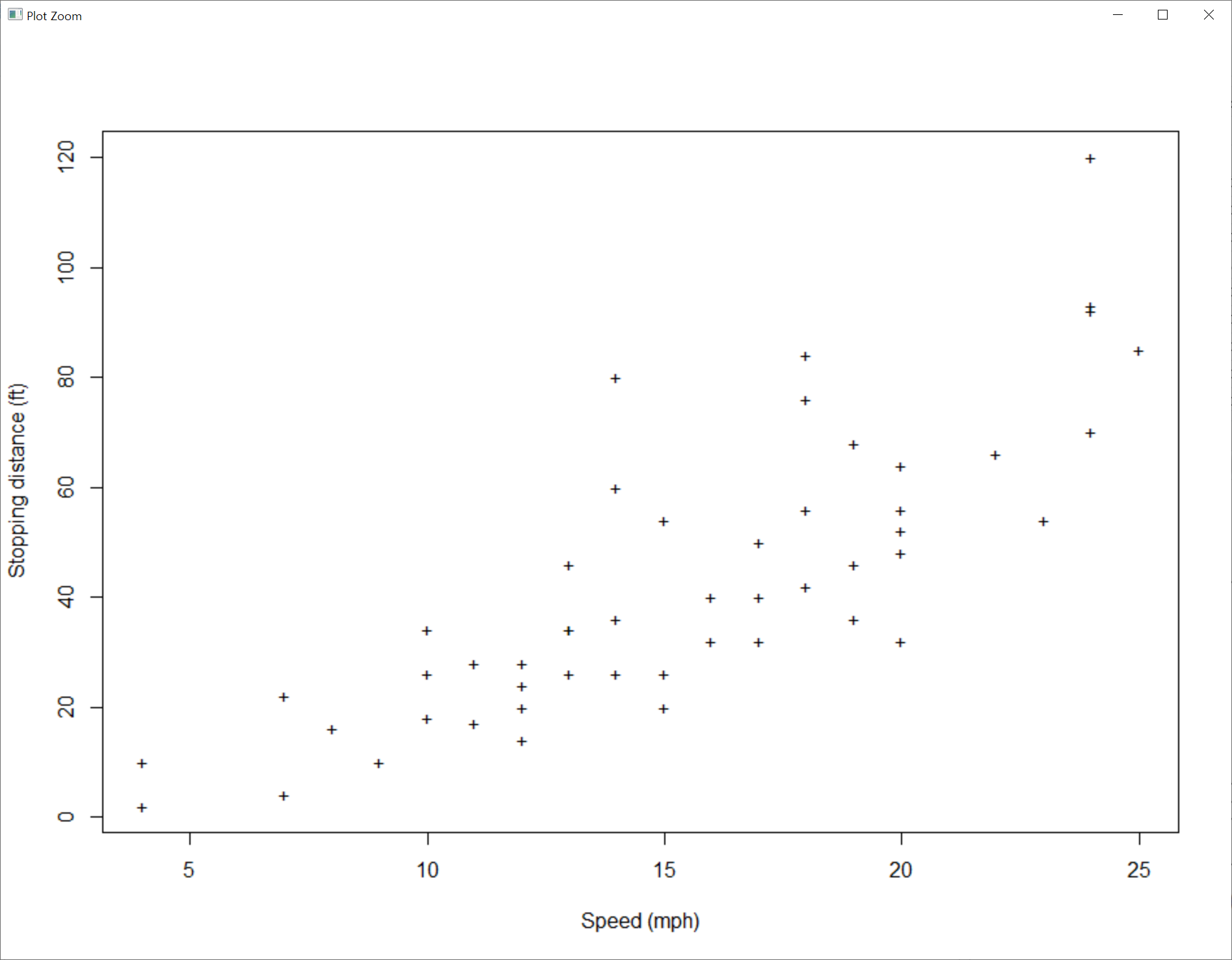
> ##### 10. 문자나 점의 크기(cex)지정 / 디폴트: cex=1 #####
> plot(dist ~ speed, xlab ="Speed (mph)", ylab ="Stopping distance (ft)",
+ pch="+", cex=1, cars)
> plot(dist ~ speed, xlab ="Speed (mph)", ylab ="Stopping distance (ft)",
+ pch="+", cars)

> plot(dist ~ speed, xlab ="Speed (mph)", ylab ="Stopping distance (ft)",
+ pch="+", cex=2, cars)
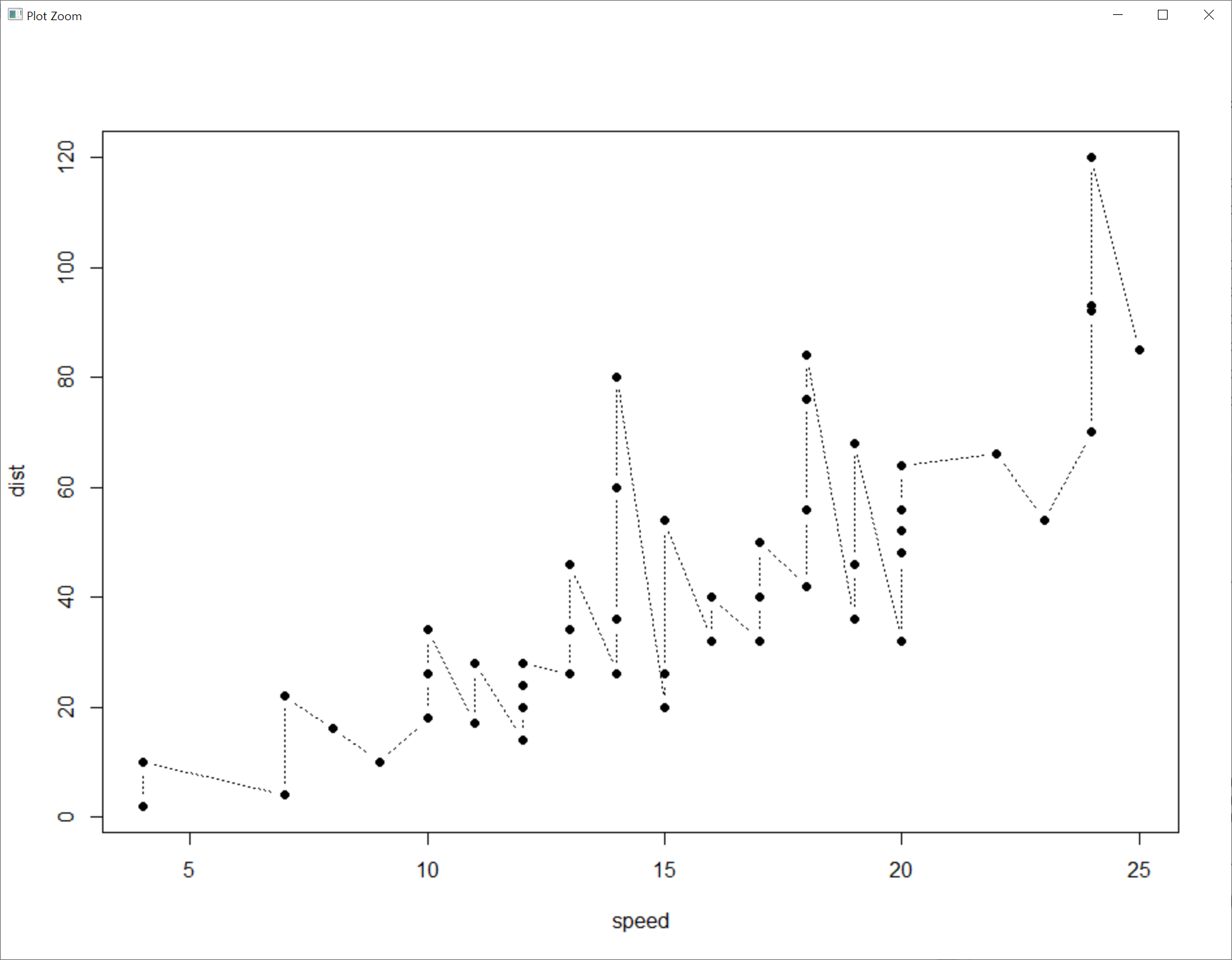
> ##### 11. par()함수를 이용한 그래픽모수 설정 #####
> plot(dist~speed, type="b", lty=3, pch=19, cars)

> opar=par(no.readonly=TRUE) # readonly=TRUE 수정이 가능한 모수들의 값들만 저장시킴
> par(lty=3, pch=19) # par() 함수로 모수 설정
> plot(dist~speed, type="b", cars)
> par(opar) # par(opar) 원래의 모수값으로 복귀
> # par()함수로 이 값을 변경하여도 plot()함수 안에서는 적용되지 않는다. 기본값인 type="p"가 적용된다.
> mypar=par(no.readonly=TRUE)
> par(mfrow=c(1,2), type="h") # 행 기준, 1행 2열로 Plots의 공간 나눔. 그래픽 파라미터 "type"은 par() 함수로 설정할 수 없음
경고메시지(들):
In par(mfrow = c(1, 2), type = "h") :
그래픽 파라미터 "type"는 필요하지 않습니다
> plot(0:5, 0:5, main="default") # type="h"가 par() 함수로 적용되지 않아 디폴트 값인 type="p"로 실행
> plot(0:5, 0:5, type ="b", main="type=\"l\" ")
> par(mypar) # 원래의 형태로 복귀

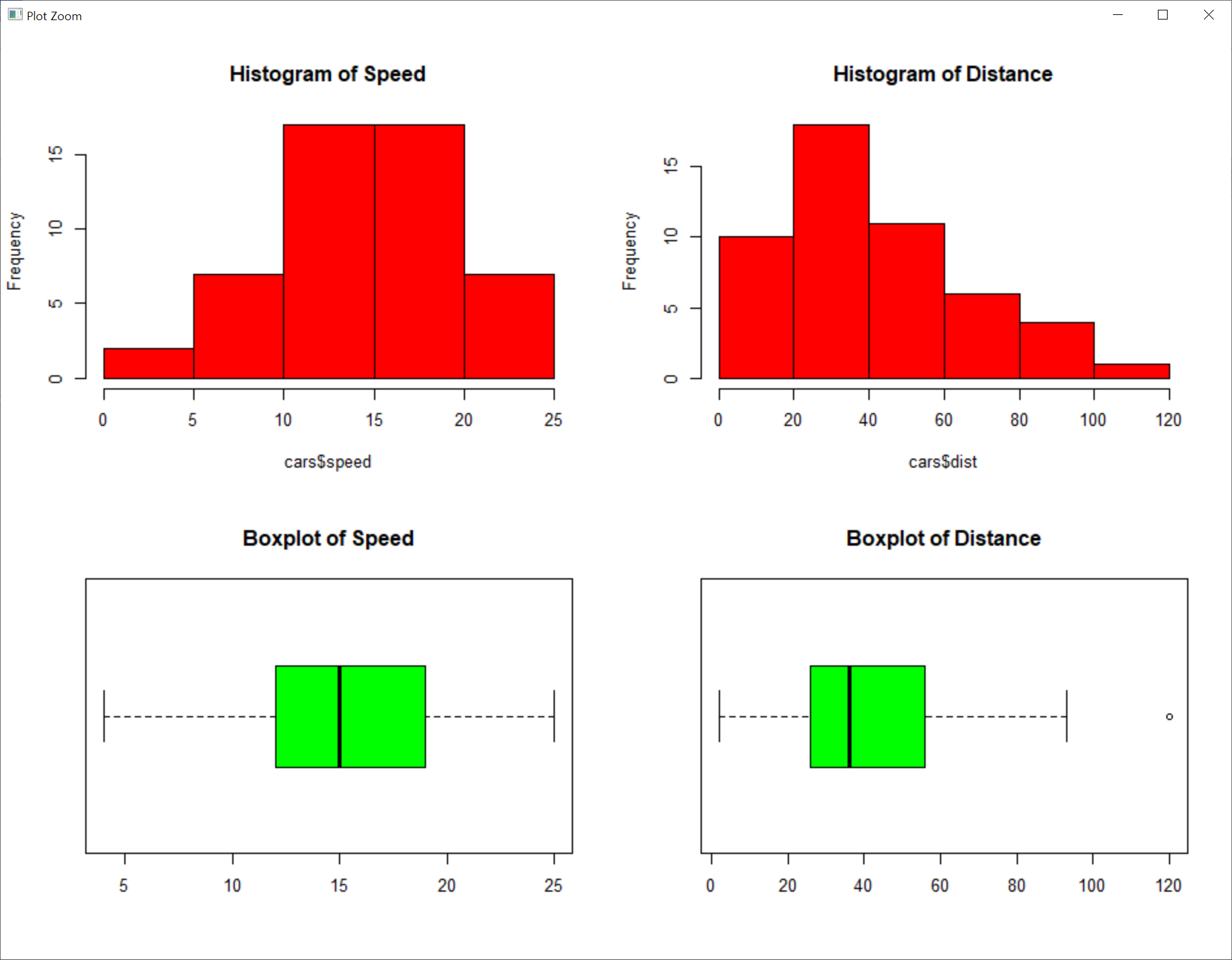
> ##### 12. mfrow, mfcol 를 이용한 플랏영역을 만들고 배치의 순서를 설정하는 인수 #####
>
> # 1) 그래프의 배열(mfcol)을 이용한 그래프 유형
> # 4 figures arranged in 2 rows and 2 columns
>
> mypar=par(mfcol=c(2, 2)) # plot 영역을 열 우선으로 하여 2행 2열로 나눔
> hist(cars$speed, main ="Histogram of Speed", col="red") # (1,1), 속도의 히스토그램
> boxplot(cars$speed, main ="Boxplot of Speed", col="green", horizontal=TRUE) # (2,1), 속도의 상자그림(수평)
> hist(cars$dist, main ="Histogram of Distance", col="red") # (1,2), 거리의 히스토그램
> boxplot(cars$dist, main ="Boxplot of Distance", col="green", horizontal=TRUE) # (2,2), 거리의 상자그림(수평)
> par(mypar)

> # 2) 그래프의 배열(mfrow)을 이용한 그래프 유형
>
> mypar <- par(mfrow=c(2,4)) # plot 영역을 행 우선으로 하여 2행 4열로 나눔
> x <- 1:6
> y <- 1:6
> plot(x, y, type ="p", main="type=\"p\" ")
> plot(x, y, type ="l", main="type=\"l\" ")
> plot(x, y, type ="b", main="type=\"b\" ")
> plot(x, y, type ="o", main="type=\"o\" ")
> plot(x, y, type ="c", main="type=\"c\" ")
> plot(x, y, type ="s", main="type=\"s\" ")
> plot(x, y, type ="S", main="type=\"S\" ")
> plot(x, y, type ="h", main="type=\"h\" ")
> par(mypar)

> ##### 13. layout()함수를 이용한 플랏영역을 만들고 배치의 순서를 설정하는 인수(확장성이 훨 더 뛰어남) #####
>
> m = matrix(c(1,2,3,4), ncol=2)
> layout(mat=m)
> hist(cars$speed, main ="Histogram of Speed", col="red")
> boxplot(cars$speed, main ="Boxplot of Speed", col="green", horizontal=TRUE)
> hist(cars$dist, main ="Histogram of Distance", col="red")
> boxplot(cars$dist, main ="Boxplot of Distance", col="green", horizontal=TRUE)
> layout(mat=c(1, 1))
> ##### 14. 좌표축 값의 범위(xlim, ylim) : par() 함수에서는 지원되지 않는 인수로 높은수준 그래픽함수에서 사용#####
>
> min(cars$speed)
[1] 4
> min(cars$dist)
[1] 2
> max(cars$speed)
[1] 25
> max(cars$dist)
[1] 120
> plot(dist ~ speed, cars, main="Speed and Stopping Distances of Cars", xlim=c(0, 25), ylim=c(0, 120))

'데이터 [Data] > R' 카테고리의 다른 글
| R Distributions: 이항분포의 누적분포함수 (0) | 2021.06.05 |
|---|---|
| R Distributions: 이항분포 (0) | 2021.06.04 |
| R Graphics 2: 그래프유형, 색상, 낮은 수준의 그래프함수 (0) | 2021.06.02 |
| R Graphics 1: plot(), attach(), with() 함수, 제목, 축 이름, 점(pch) (0) | 2021.06.01 |
| R apply 함수군: apply(), lapply(), sapply(), tapply(), mapply() (0) | 2021.05.01 |


댓글